As a general rule we do four analyses fairly commonly in the Bridges Lab, summarized here based on the nature of the independent and dependent variables:
Dependent Variable
Independent Variable
Analysis
Continuous
Continuous
Linear Regression
Continuous
Counts (Yes/No or Groups)
Pairwise Test (t-test/Mann-Whitney/ANOVA)
Counts (Yes/No or Groups)
Continuous
Binomial Regression
Counts (Yes/No or Groups)
Counts (Yes/No or Groups)
\(\chi^2\) or Fisher’s Test
Lets take a Bayesian approach to each of these using the Mtcars dataset, which looks like this after a bit of fiddling.
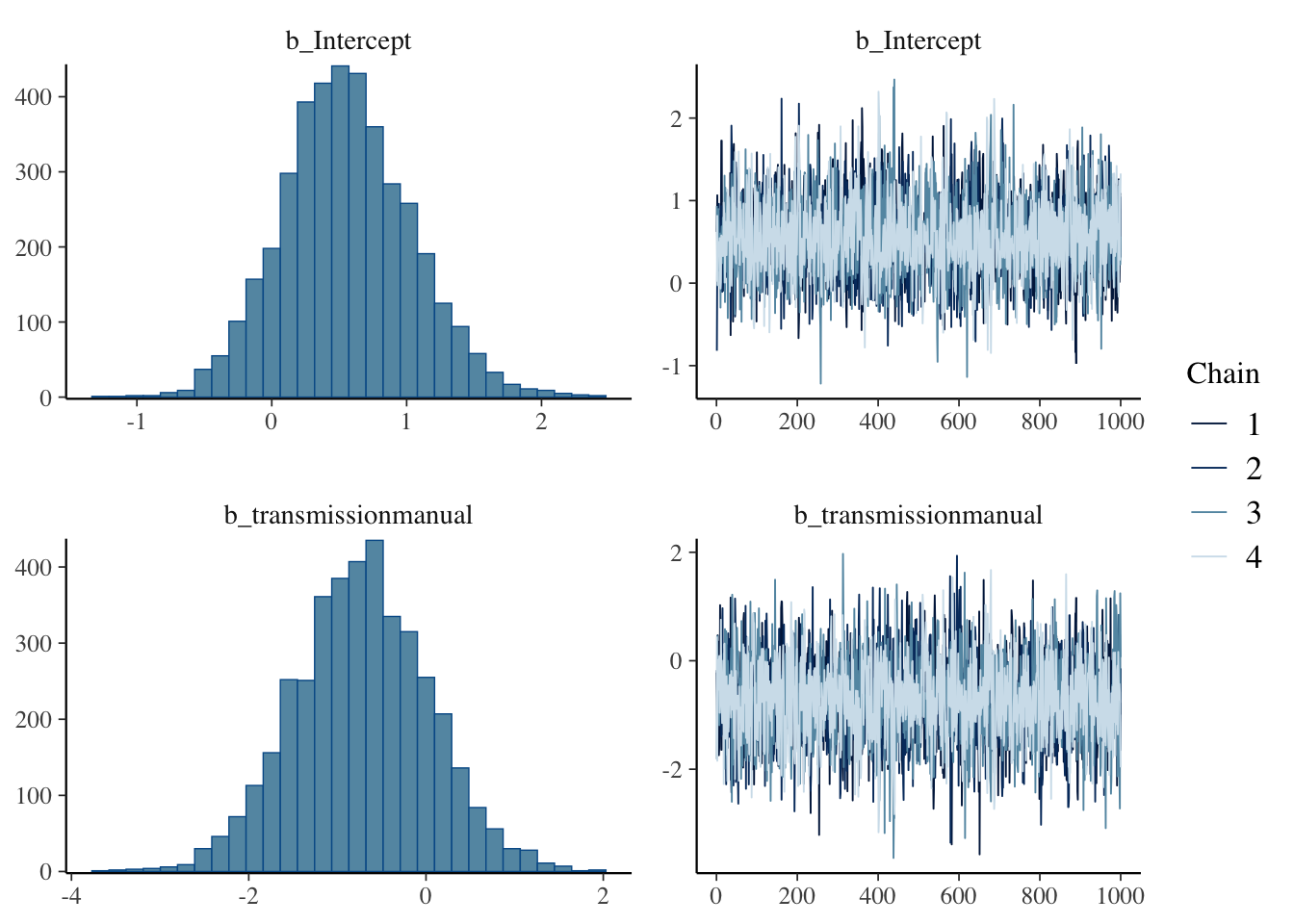
Let’s start by testing if there is a relationship between a quantitative variable — mpg (miles per gallon) — and a categorical variable — transmission (manual or automatic) — using the default priors.
library(brms)# directory for cached model fits — brms reuses these on re-renderdir.create("fits", showWarnings =FALSE)pairwise.fit <-brm(mpg~transmission,data=mtcars.data,sample_prior =TRUE,file ="fits/mtcars-pairwise",file_refit ="on_change")
library(broom.mixed)tidy(pairwise.fit) %>%kable(caption="Summary of model fit for mpg versus transmission")
Summary of model fit for mpg versus transmission
effect
component
group
term
estimate
std.error
conf.low
conf.high
fixed
cond
NA
(Intercept)
17.113379
1.1689889
14.7144609
19.399643
fixed
cond
NA
transmissionmanual
7.269073
1.8365570
3.5006106
10.800207
ran_pars
cond
Residual
sd__Observation
5.044648
0.6506777
3.9783786
6.482545
ran_pars
cond
Residual
prior_sigma__NA.NA.prior_sigma
5.992310
6.9772388
0.1794762
23.392327
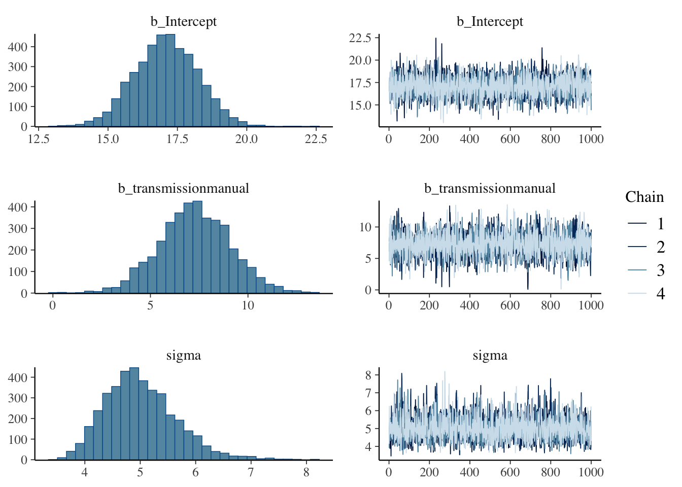
plot(pairwise.fit)
hypothesis(pairwise.fit, "transmissionmanual>0") # testing whether manual transmission has higher mpg
Hypothesis Tests for class b:
                Hypothesis Estimate Est.Error CI.Lower CI.Upper Evid.Ratio
1 (transmissionmanual) > 0     7.27      1.84     4.23    10.28        Inf
  Post.Prob Star
1         1    *
---
'CI': 90%-CI for one-sided and 95%-CI for two-sided hypotheses.
'*': For one-sided hypotheses, the posterior probability exceeds 95%;
for two-sided hypotheses, the value tested against lies outside the 95%-CI.
Posterior probabilities of point hypotheses assume equal prior probabilities.
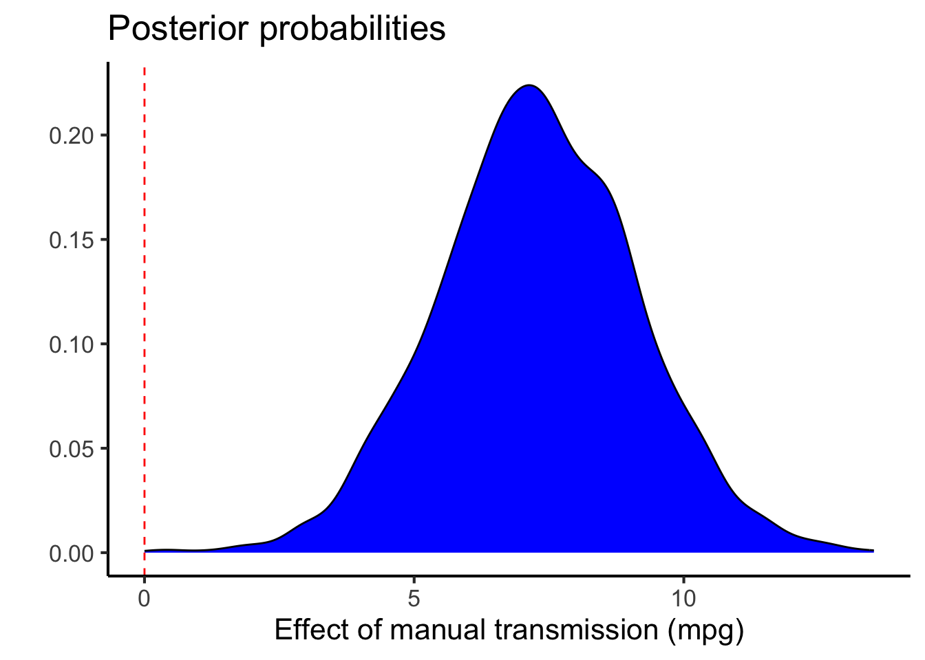
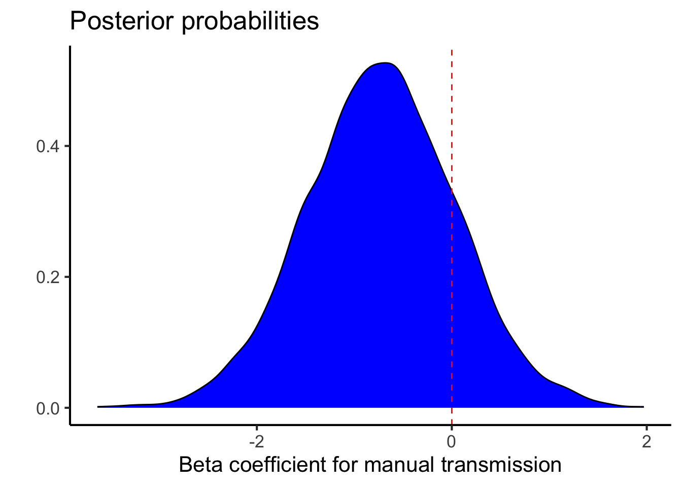
As you can see, this analysis estimates that the manual transmission has a 7.2690725 higher mpg (\(\pm\) 1.836557) with a very high Bayes Factor () and posterior probability (1).
The posterior distribution for the effect of a manual transmission is here:
We didn’t specify the model type (Gaussian is the default). We also used the default priors here, which were
prior_summary(pairwise.fit) %>%kable(caption="Default priors for a pairwise analysis of mpg vs transmission in the mtcars data")
Default priors for a pairwise analysis of mpg vs transmission in the mtcars data
prior
class
coef
group
resp
dpar
nlpar
lb
ub
tag
source
b
default
b
transmissionmanual
default
student_t(3, 19.2, 5.4)
Intercept
default
student_t(3, 0, 5.4)
sigma
0
default
This includes flat priors for the beta coefficients, student’s t distributions for intercept (centered around the mean mpg) and residual error (centered around zero).
How about an ANOVA
Let’s say we want to test across groups (rather than testing effects between two groups). For that we can use the number of cylinders as a factor.
Important note on Bayes factors with default priors:bayes_factor() uses bridge sampling to estimate marginal likelihoods, which requires proper (integrable) priors on every parameter. The default brms priors include flat (improper) priors on the beta coefficients — under those priors the marginal likelihood is undefined and any number bayes_factor() returns is unreliable. So before doing model comparison we need to set proper priors explicitly.
anova.priors <-c(prior(normal(20, 10), class = b), # weakly informative on cylinder meansprior(student_t(3, 0, 5), class = sigma))anova.fit <-brm(mpg ~0+ cylindars, data = mtcars.data, # zero gives each cylinder its own interceptprior = anova.priors,sample_prior =TRUE,save_pars =save_pars(all =TRUE), # required for bayes_factor()file ="fits/mtcars-anova",file_refit ="on_change")# Null model: a single intercept (no cylinder effect). Use the same proper prior# class so the marginal likelihood is well-defined.anova.fit.null <-brm(mpg ~1, data = mtcars.data,prior =c(prior(normal(20, 10), class = Intercept),prior(student_t(3, 0, 5), class = sigma)),sample_prior =TRUE,save_pars =save_pars(all =TRUE),file ="fits/mtcars-anova-null",file_refit ="on_change")
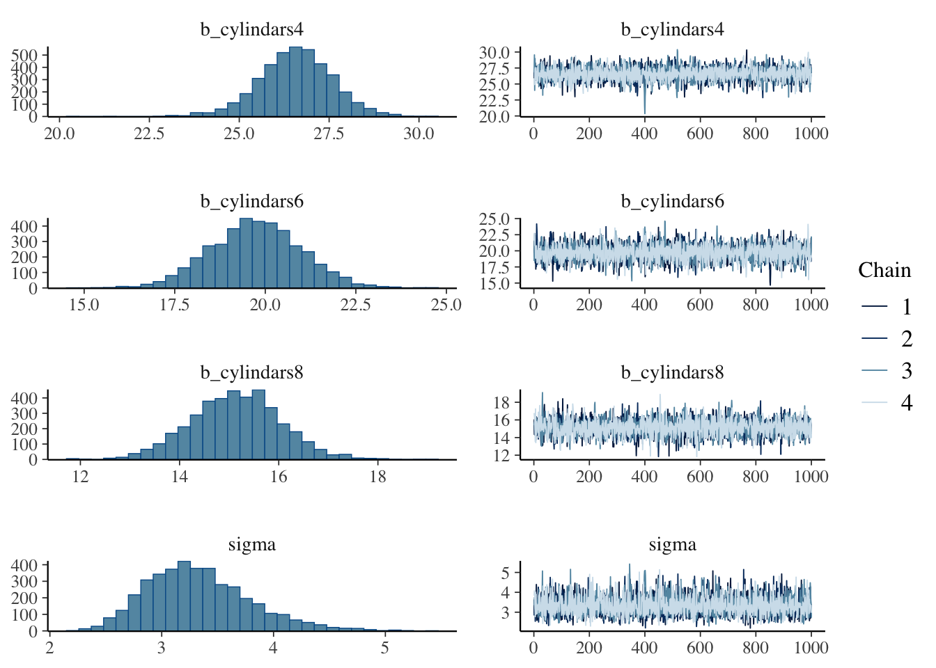
The analysis here is a little different than before. We can still plot the posterior distributions for each model but the relevant test is now to compare the model with cylinders to a null model without that term.
tidy(anova.fit) %>%kable(caption="Summary of model fit for mpg versus cylinders")
Summary of model fit for mpg versus cylinders
effect
component
group
term
estimate
std.error
conf.low
conf.high
fixed
cond
NA
cylindars4
26.571554
1.0218075
24.4738104
28.529332
fixed
cond
NA
cylindars6
19.734955
1.2593976
17.3189086
22.169466
fixed
cond
NA
cylindars8
15.138110
0.9067475
13.3600901
16.914190
ran_pars
cond
Residual
sd__Observation
3.333054
0.4632648
2.5615760
4.380818
ran_pars
cond
Residual
prior_sigma__NA.NA.prior_sigma
5.554511
6.2958228
0.1703158
20.330537
plot(anova.fit)
# extracts the bayes factor comparing the models (well-defined now that priors are proper)bayes_factor(anova.fit, anova.fit.null) -> anova.bf
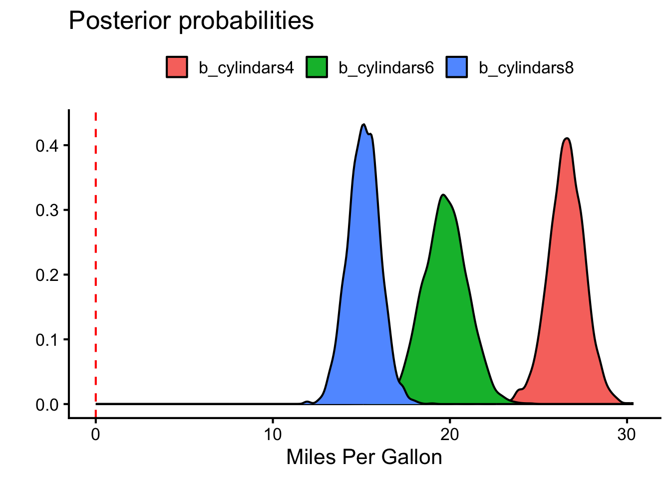
In this case the Bayes Factor for the hypothesis that the cylinder term is relevant is 8.7851778^{6}.
We can still do post-hoc tests using the hypothesis command:
rbind(hypothesis(anova.fit, "cylindars4>cylindars6")$hypothesis,hypothesis(anova.fit, "cylindars4>cylindars8")$hypothesis,hypothesis(anova.fit, "cylindars6>cylindars8")$hypothesis) %>%kable(caption="Pairwise hypothesis tests for cylinders on mpg")
Pairwise hypothesis tests for cylinders on mpg
Hypothesis
Estimate
Est.Error
CI.Lower
CI.Upper
Evid.Ratio
Post.Prob
Star
(cylindars4)-(cylindars6) > 0
6.836599
1.604323
4.131769
9.397150
3999
0.99975
*
(cylindars4)-(cylindars8) > 0
11.433444
1.362242
9.188783
13.678269
Inf
1.00000
*
(cylindars6)-(cylindars8) > 0
4.596845
1.587968
2.064742
7.192442
499
0.99800
*
What is a Linear Regression Equivalent?
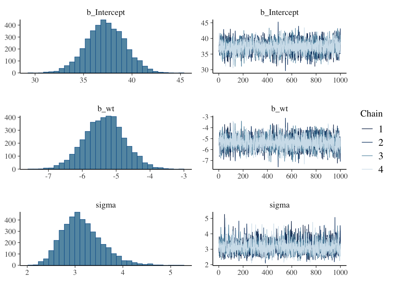
Lets start by testing if there is a relationship between two quantitative variables, the mpg (miles per gallon) and the weight (wt) using the default priors
prior_summary(linear.fit) %>%kable(caption="Prior summary for effects of weight on mpg")
Prior summary for effects of weight on mpg
prior
class
coef
group
resp
dpar
nlpar
lb
ub
tag
source
b
default
b
wt
default
student_t(3, 19.2, 5.4)
Intercept
default
student_t(3, 0, 5.4)
sigma
0
default
tidy(linear.fit) %>%kable(caption="Summary of model fit for mpg versus weight")
Summary of model fit for mpg versus weight
effect
component
group
term
estimate
std.error
conf.low
conf.high
fixed
cond
NA
(Intercept)
37.332230
1.9906229
33.3489093
41.294963
fixed
cond
NA
wt
-5.358417
0.5981328
-6.5391982
-4.204272
ran_pars
cond
Residual
sd__Observation
3.151748
0.4136588
2.4693176
4.049447
ran_pars
cond
Residual
prior_sigma__NA.NA.prior_sigma
5.955288
6.6215206
0.1628139
21.955359
plot(linear.fit)
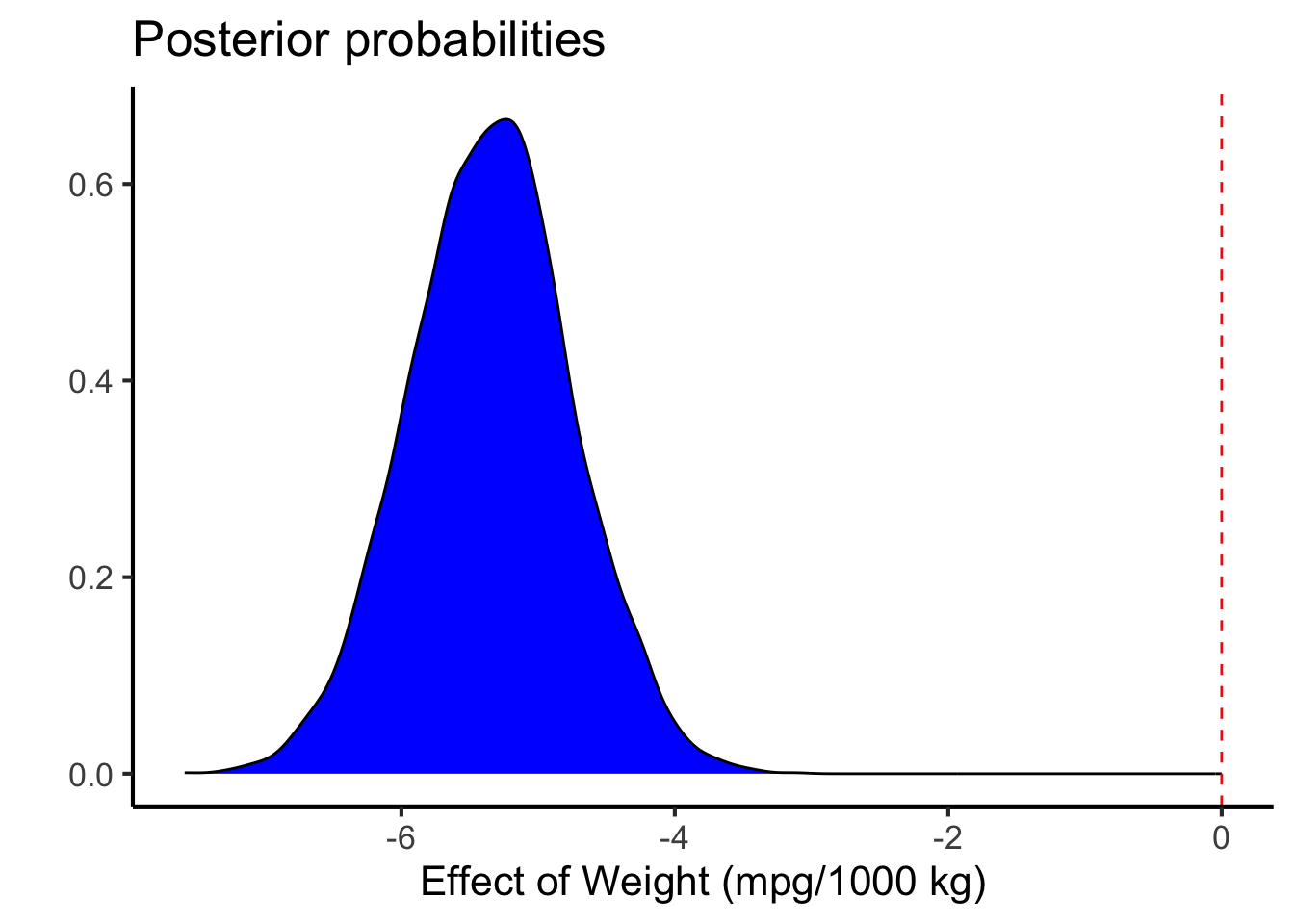
hypothesis(linear.fit, "wt<0") # testing for whether weight has a negative effect on mpg
Hypothesis Tests for class b:
  Hypothesis Estimate Est.Error CI.Lower CI.Upper Evid.Ratio Post.Prob Star
1   (wt) < 0    -5.36       0.6    -6.32    -4.38        Inf         1    *
---
'CI': 90%-CI for one-sided and 95%-CI for two-sided hypotheses.
'*': For one-sided hypotheses, the posterior probability exceeds 95%;
for two-sided hypotheses, the value tested against lies outside the 95%-CI.
Posterior probabilities of point hypotheses assume equal prior probabilities.
Notice that the priors were the same here (they are based on the dependent variable), and again there is a highly probable inverse relationship between mpg and weight (heavier cars get lower fuel economy).
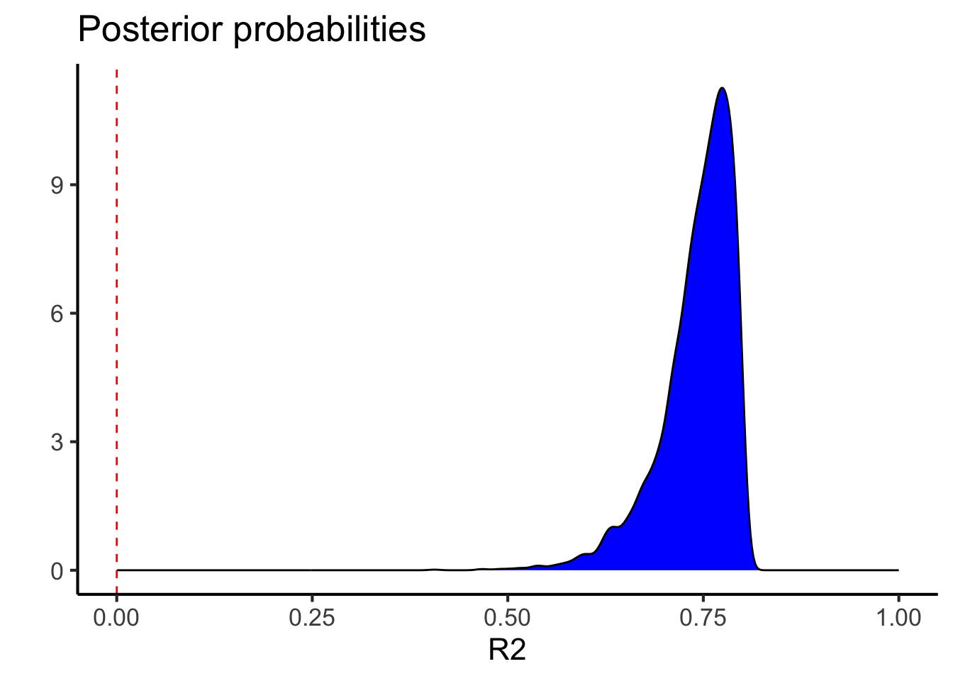
What if I am more interested in the R-squared?
To do this we can use the bayes_R2 function.
kable(bayes_R2(linear.fit),caption="Estimates for R2 between weight and mpg")
Estimates for R2 between weight and mpg
Estimate
Est.Error
Q2.5
Q97.5
R2
0.7422678
0.0472943
0.6234056
0.7982604
r2.probs <-bayes_R2(linear.fit, summary=F) #summary false is to get the posterior probabilitiesggplot(data=r2.probs, aes(x=R2)) +geom_density(fill="blue") +geom_vline(xintercept=0,color="red",lty=2) +labs(y="",x="R2",title="Posterior probabilities") +lims(x=c(0,1)) +theme_classic(base_size=16)
What is a Chi-Squared Equivalent
First let’s do an example with a standard \(\chi^2\) test (and a Fisher’s test since the counts are quite low) on whether there is a relationship between engine type and transmission type.
library(tidyr) #for pivot widerlibrary(tibble) #for column to rownameengine.trans.counts <- mtcars.data %>%group_by(engine,transmission) %>%count() %>%pivot_wider(names_from=transmission,values_from=n) %>%column_to_rownames('engine')chisq.test(engine.trans.counts) %>% tidy %>%kable(caption="Chi-squared test for engine/transmission")
Chi-squared test for engine/transmission
statistic
p.value
parameter
method
0.3475355
0.5555115
1
Pearson’s Chi-squared test with Yates’ continuity correction
fisher.test(engine.trans.counts) %>% tidy %>%kable(caption="Fisher's test for engine/transmission")
Fisher’s test for engine/transmission
estimate
p.value
conf.low
conf.high
method
alternative
0.511233
0.4726974
0.0944144
2.614145
Fisher’s Exact Test for Count Data
two.sided
Both agree, not much of a relationship here. For the brms modelling we need to make a few changes. First, we will use a bernoulli distribution since our data is only zeros and ones, again we will use all the default priors.
# Fit the modelcounts.model <-brm(engine ~ transmission,data = mtcars.data,family =bernoulli(),file ="fits/mtcars-engine-transmission",file_refit ="on_change")
Lets look at these results
prior_summary(counts.model) %>%kable(caption="Prior summary for effects of transmission on engine type")
Prior summary for effects of transmission on engine type
prior
class
coef
group
resp
dpar
nlpar
lb
ub
tag
source
b
default
b
transmissionmanual
default
student_t(3, 0, 2.5)
Intercept
default
tidy(counts.model) %>%kable(caption="Summary of model fit for transmission versus engine type")
Summary of model fit for transmission versus engine type
effect
component
group
term
estimate
std.error
conf.low
conf.high
fixed
cond
NA
(Intercept)
0.5613834
0.4767499
-0.3517906
1.5203421
fixed
cond
NA
transmissionmanual
-0.7442098
0.7650699
-2.2922495
0.7335985
plot(counts.model)
hypothesis(counts.model, "transmissionmanual<0") # testing whether manual transmission decreases the log-odds of a V-shaped engine
Hypothesis Tests for class b:
                Hypothesis Estimate Est.Error CI.Lower CI.Upper Evid.Ratio
1 (transmissionmanual) < 0    -0.74      0.77    -2.04     0.48        5.3
  Post.Prob Star
1      0.84
---
'CI': 90%-CI for one-sided and 95%-CI for two-sided hypotheses.
'*': For one-sided hypotheses, the posterior probability exceeds 95%;
for two-sided hypotheses, the value tested against lies outside the 95%-CI.
Posterior probabilities of point hypotheses assume equal prior probabilities.
Now in this case there is moderate evidence for a negative relationship between transmission and engine type (\(\beta\)=-0.7442098 \(\pm\) 0.7650699) with a Bayes Factor of 5.2992126 and a Posterior Probability of 0.84125.
What is a Binomial Regression Equivalent?
Let’s now look at the relationship between transmission type (binomial variable) and weight (continuous variable). Again we will use a Bernoulli distribution (which uses a logit link function by default).
# Fit the modelbinomial.fit <-brm(transmission ~ wt,data = mtcars.data,family =bernoulli(),file ="fits/mtcars-binomial",file_refit ="on_change")
prior_summary(binomial.fit) %>%kable(caption="Prior summary for effects of transmission on engine type")
Prior summary for effects of transmission on engine type
prior
class
coef
group
resp
dpar
nlpar
lb
ub
tag
source
b
default
b
wt
default
student_t(3, 0, 2.5)
Intercept
default
tidy(binomial.fit) %>%kable(caption="Summary of model fit for transmission versus engine type")
Summary of model fit for transmission versus engine type
effect
component
group
term
estimate
std.error
conf.low
conf.high
fixed
cond
NA
(Intercept)
14.457099
5.012188
6.401645
25.648173
fixed
cond
NA
wt
-4.788294
1.594304
-8.385464
-2.204216
plot(binomial.fit)
hypothesis(binomial.fit, "wt<0") # testing whether weight decreases the log-odds of a manual transmission
Hypothesis Tests for class b:
  Hypothesis Estimate Est.Error CI.Lower CI.Upper Evid.Ratio Post.Prob Star
1   (wt) < 0    -4.79      1.59     -7.6    -2.51        Inf         1    *
---
'CI': 90%-CI for one-sided and 95%-CI for two-sided hypotheses.
'*': For one-sided hypotheses, the posterior probability exceeds 95%;
for two-sided hypotheses, the value tested against lies outside the 95%-CI.
Posterior probabilities of point hypotheses assume equal prior probabilities.
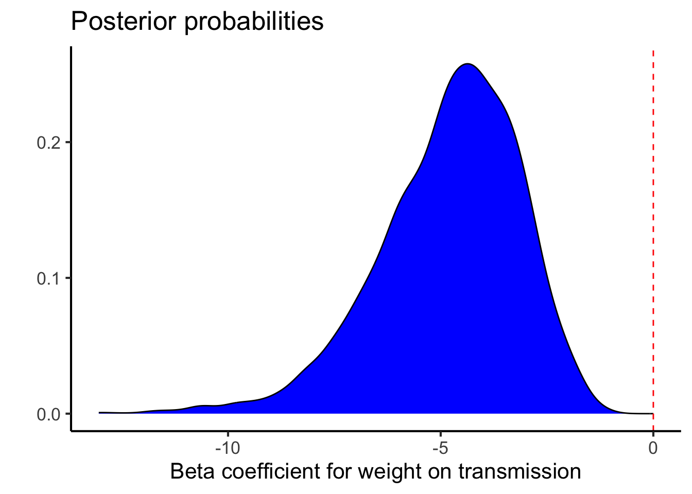
as_draws_df(binomial.fit) %>%ggplot(aes(x=b_wt)) +geom_density(fill="blue") +geom_vline(xintercept=0,color="red",lty=2) +labs(y="",x="Beta coefficient for weight on transmission",title="Posterior probabilities") +theme_classic(base_size=16)
Again there is strong evidence that a higher weight makes an automatic transmission more likely.
Hopefully these examples helped, but a couple things since we used defaults.
Think closely about your priors, if you have a good reason to set them to something other than the default you should. In this case the defaults worked pretty well and as you can see are set based on the data that is input. These are generally very weakly informative priors and the modelling could be improved on by setting your own.
Also remember, nowhere in here was there a p-value. We could consider a posterior probability of >0.95 our cutoff for significance if we prefer, but make sure to state this in your methods (along with your choice of priors and the package used.)
Note this script used some examples generated by perplexity.ai and then modified further